2 years from the last Cube Project post,
some of you might be expecting
this third edition to come out sooner or later.
The Idea
So far, I have had a single project related to the cube every single year;
the Speedcube Method Efficiency Analysis project
in first year as part of Science One,
and the Cube Timer project in second year as part of CPSC 210.
Naturally, it would be ingenious to continue the theme
and work on a cube-related project in third year.
As such, as part of PHYS 319, an electronics lab course,
I have chosen to build a microcontroller-based robotic Rubik’s Cube solver.
The Parts
Stepper Motor
Since we would need to individually move the 6 faces of the cube,
we would need motors that have precise positional control,
with the additional benefit that
they can turn an indefinite amount in any direction.
Our choice is the use 6 stepper motors,
specifically the NEMA 17 bipolar stepper motors,
which you can often find for a cheap price on Amazon.
Bipolar stepper motors operate on two coils,
and given a current alternately between the coils,
we can drive the motor shaft (a permanent magnet) to rotate a precise angle,
and in our case exactly 1.8°.
Stepper Motor Driver
However, the delicate task of controlling a single stepper motor
requires four output pins on the microcontroller,
which adds up to 24 output pins to control six motors,
taking up a significant amount of the total available pins.
Therefore, we delegate the task of manouvering a stepper motor
to a specialized integrated circuit, the stepper motor driver,
which requires significantly fewer pins to control..
The cheapest and most common drivers found on Amazon are the A4988,
which we need one each for the six stepper motors.
Now they would only require 3 signals each to control,
2 of which can be the same signal between all drivers.
Coupling Mechanism
Now that we have the thing that moves (the motor)
and the thing that is about to be moved (the cube),
we need to figure out a way to connect those two parts.
Since there is no premade component that interfaces a cube and a motor,
we must therefore design our own.
To successfully turn the face of a cube,
we merely need to turn the center of the cube.
Our mechanism relies on the cube having detachable center tiles,
which we can slot in our mechanism that grapples on it.
This cubeside part must be connected to the motorside part
such that as the motor shaft rotates,
the parts rotate along with it.
We have designed these two parts to be separable
so that we gain the possibility and convenience of
removing the cube itself without disturbing the motor setup.
A small thank you to Morgan for lending me his 3D printer,
which made the production of these parts possible.
Power Supply
The next issue is with a power supply.
Since the logic voltage supply is usually either 3.3V or 5V,
while the motor voltage supply needs to be above 8V,
we must use different power supplies for the logic and motor circuits.
As motors can often draw a lot of current and power,
to minimize heat dissipation,
we have chosen the logic voltage as 3.3V,
and the motor voltage to be 12V.
Although the motors themselves are rated at 7.3V,
we can tune the potentiometer on the driver itself
such that no excessive voltage or current will go through the motor.
The choice of 12V is also partly due to the cube itself.
Inside every single center,
there is a tunable spring.
If we let the spring be more loose,
then we would require a lower torque to overcome static friction,
and hence the motor would not require as much power and voltage;
however, the faces of the cube will cam outwards as we rotate them,
which might lead to small undesired movements of the cube itself,
and the faces might get stuck in the middle of a rotation,
potentially leading to a rapid disassembly of both the cube and the machine.
On the other hand,
to prevent that from happening,
we woudl require a higher torque to overcome the higher static friction,
and hence the motor would require more power and higher voltage.
Our final choice of 12V and 1.3A is a good balance.
Before successfully sourcing for a potential power supply,
I have been using the AC to 12V that came with the Wi-Fi router at home.
Luckily, I had found an identical power supply in Best Buy
merely days before the actual presentation for this project,
as otherwise my home would have to go without internet
every time I try to power up my robot.
Structure
To package together all the components,
we must build a frame.
We used a Lego set that is readily available,
which allowed for quick prototyping of different structures
at the cost of a small amount of precision of placements.
The other obvious choice for the material for the structure
would be laser-cut acrylic sheets.
This would have been the preferred way to build the structure,
as I am familiar with laser cutters from grades 7 & 8;
however, I did not know that we had access to the laser cutters,
which were just situated in the engineering physics lab next door.
The Logic
Microcontroller
As the microcontroller itself lacks the computing power
to perform a search to find a solution,
we can outsource this to a host computer,
so the only task the microcontroller really needs to perform
is to receive instructions from the host computer
and then execute those instructions on the motors.
We have chosen to use
the universal asynchronous transmitter-receiver (UART) protocol,
and as its name suggests,
is a universal protocol for two-way communication.
Both sides can initiate a message transmission,
which is a desired function,
as we want the host computer to raise an interrupt flag
on the microcontroller side when we send in a move instruction,
allow the microcontroller to perform that move,
and let it raise an interrupt flag on the host computer in return
as to signal that it has completed the move,
and is ready to receive another instruction.
As UART can only send one byte at a time,
we can encode information about which motor needs to move
and the amount it needs to move by in eight bits, or two hexits.
We let the most significant hexit range from 0 to 5,
representing the pin that we will enable,
and therefore the motor that we will activate;
and we let the least significant hexit range from 0 to 2,
representing 90° clockwise, 180°, and 90° counterclockwise
movements respectively.
The typical cycle of communication looks like the following:
Microcontroller receives a single instruction via UART.
Decodes it into our desired motor and movement.
Activate corresponding motor and change directions.
Step the motor the desired number of times.
Disable motor.
Signal to host computer that movement is complete via UART.
Host Computer
However, we must generate those set of moves
before we can send it to the microcontroller.
This is written in Python,
as Python has a package for serial port communication via UART,
and also a twophase package for Rubik’s cube solving.
All we have to do is to input the 54 colours of the cube,
allow time for the computer to find a solution,
encode these moves into hexits,
and then send them one by one via UART.
The Algorithm
Well then, one might ask,
what algorithm might we want to use to solve the cube?
We already had one such discussion in part 1,
but that mostly pertains to human solvers,
which are very limited in memory and search speed.
We could try to implement CFOP or Roux deterministically as we did back then,
but number of lookup tables involved there are minimal,
which implies we would not be taking the most advantage of the computer.
We now turn our attention to
Kociemba’s algorithm.
Created by Herbert Kociemba in 1992,
this is an algorithm that solves the Rubik’s cube in two phases.
Let us first define two groups,
$G_0 = \langle U,D,L,R,F,B \rangle$
and $G_1 = \langle U,D,L^2,R^2,F^2,B^2 \rangle$.
For those unfamiliar with abstract algebra,
we can treat $G_0$ as the set of cube states that we can get to
(note that we are equating sequence of moves applied to starting cube state
to the cube state itself)
by applying any composition of the moves ${U,D,L,R,F,B}$ to the cube
(i.e. all possible states);
and similarly, $G_1$ is also a set of cube states,
but given its generating set of moves are more restrictive,
it is a smaller set of possible states,
and in fact is a normal subgroup of $G_0$.
An easy description of $G_1$ would be that
the orientation of all edges and corners are solved,
and the 4 edges between the $U$ and $D$ slices are within that slice.
Side note.
As we noted earlier, we are treating the moves and the cube states
as the same exact group.
Formally speaking, the group of moves $G_0$
acts on a set $G_0$ of all possible legal cube states,
with correct spin and parity.
Choosing the starting state of a solved cube $1 \in G_0$,
the orbit of $1$ under $G_0$,
defined as the set of all possible cube states in $G_0$ (the set)
that we can obtain by applying the moves in $G_0$,
must be the entire set $G_0$.
The first phase of the algorithm searches through the coset space $G_0/G_1$,
that is, trying to find a solution that gets us to a cube state in $G_1$.
By exhausting through all possibilities in this state,
we can generate lookup tables that also serve as a heuristic function
for the search function,
which helps us evaluate which moves we should try first.
Moreover, the generated lookup tables
allow us to prune away large amounts of incorrect moves,
reducing the computation time at the cost of memory.
The second phase of the algorithm now continues the search
using only the moves ${U,D,L^2,R^2,F^2,B^2}$,
permuting through the possible locations for each piece.
Notice that we do not terminate the algorithm at the first complete solution;
we will now continue to search the second phase
by using less optimal solutions in the first phase.
Suppose we originally needed $n$ moves in the first phase,
and $m$ moves in the second phase.
After we have found this solution,
we will now proceed to a suboptimal solution of $n+1$ moves in the first phase,
and attempt to find a solution of less than $m-1$ moves in the second phase.
We repeat this process until $m=0$,
which implies we have found an optimal solution.
As we only need to find a relatively good solution
and not the absolute optimal one,
we can terminate the search early.
This is a balance between computation time and solve time.
End Result
After assembling everything together,
the final product is one such video.
Sometimes I sing in the shower. I can sometimes hear the echo when I hit particular notes.
The lowest note that I can sing, while simultaneously able to hear the reverbations is an A, 220Hz. We can model the shower room as an open-closed tube, in which resonant frequencies can be determined from the equation $f = \frac{nv}{4L}$, where $n$ is an odd number, $v$ is the speed of sound, and $L$ is length of tube. We know that the temperature inside the shower room is slightly higher than 25°C, so the speed of sound is expected to be slightly higher than 343m/s.
We can rearrange the equation to get $v = \frac{4fL}{n}$. Knowing that the glass panels that make up the shower room walls are 78” tall, we can convert that back to metric and say L = 1.98m. Plugging in n = 5 will obtain us a value of 348.5m/s.
From the textbook University Physics I found on OpenStax, equation 17.3.7 states that the speed of sound of air at sea level is about $v = 331 \sqrt{\frac{T}{273}}$, where T is temperature in Kelvins. Rearranging the equation gives us $T = 273 (\frac{v}{331})^2$, which evaluates to 303K = 30°C.
Now I know the ambient temperature of the shower room without using a thermometer, even though bringing in a thermometer is clearly a lot quicker.
As an enjoyer of different genres of music, I would like share with you a very satisfying chord progression that never fails to amaze me whenever I listen to it.
Note: Due to the lack of HTML support for the half-sharp/flat symbols, I will be using ½♯ & ½♭ to denote them.
Some Theory
In classical music theory, a very common musical cadence is the ii-V-I, where chords traverse counterclockwise two steps to the tonic chord. This brings the listener a sense of closure, a sense of “home”. Given the key of C major, we would travel Dmin-G(7)-C; in the key of A major, Bmin-E(7)-A; you get it.
Another way of providing harmonic motion, or traversing the circle of fifths, is to use chromaticism. By moving to neighbouring tones, one is making a large leap on the circle of fifths.
The Progression
The music I want to share with you is Sevish’s Gleam, which is an electronic piece that uses 22-tone equal temperament and a 5/4 beat.
Western classical music currently divides the octave into 12 steps; Gleam here divides it into 22. This allows us to get almost double the notes in an octave, with notes that can “fill in the gap” between semitones.
Said chord progression starts at 0:54. The idea is very simple: a descending chromatic, leaving the listener wondering where the destination is, and then hitting them with a V-I to signify arrival. However, as mentioned above, with the use of 22-TET, chromatic scales can mean descending in almost quarter tones.
Coupled with an ascending chromatic line above, we get a peculiar soundscape that is rarely heard: C½♯min - C9(omit7) - B½♯(½♯9) - B - B½♭7(♯9) - E - B♭7 - A(♯11). I have bolded the chords that follow the classical ii-V-I motion: they act as a reminder to the listener, bringing a tinge of familiarity as to not make 22-TET completely alien.
Now that we’ve got an idea of what I have been doing in the past few months, let us dive deep into the process of this project, from the conception of the idea, to the completed paper on the previous post.
The Idea
Not long after we finished our term 1 projects, we were tasked with finding a topic of research/measurement for our term 2 projects. If you have read my posts here, you would know that I spent my Christmas break playing Minecraft instead.
About a week before we had to submit our topics for scrutiny, I sat down and realized that I had to either find a partner who already has an idea, or come up with an original one myself. Of course the former would be preferable, since I would save time by not needing to brainstorm; but after sifting through all the available proposals, it was either that I was not interested enough in the topic, or they already have found a partner.
I needed to find a topic that is physics/math related, and preferably easy data taking, because I did not want to go outdoors. I looked around my room, and after a solid minute, landed my sights on my Rubik’s cube, which I have not touched in the past 5 years. A project idea that is unconventional, all code-based; modelling and measuring the solves of a Rubik’s cube.
Getting a partner on board with the idea was relatively easy. Callum, being a fellow cuber, hardly needed any convincing. All that was left was to plan out our project, and execute that plan.
The Metric
The premise of our project was to measure the speed of different solving methods, taking into account human factors. But first, we have to find a way to measure this speed, because every human is different, and we have to somehow standardize a time-unit for moves.
The most obvious move is to start with pre-existing measurement systems. The common ones include the quarter-, half-, and slice-turn metrics. Out of the three, the quarter-turn metric is the most unrealistic one when measuring speed, since we know cubers tend to move fluidly. We also know, from “rigourous” testing, that slice turns are slightly slower than face turns, but do not take more than double the time. Since HTM treats slice turns as 2, and STM treats them as 1, we know that STM will inherently favour methods that utilize slice turns, while HTM will favour otherwise. However, to avoid working with decimals in code, we have decided to stick with these two metrics rather than to come up with one that treats slice turns as something between 1 & 2.
No matter how sophisticated counting slice turns are, they unfortunately do not take into account any other huamn-related factor. This leads to the incorporation of the 4 different factors: deduction, regrips, rotations, and look time. As explained in the previous post, the two different adjustments that we made to these pre-existing metrics are a combination of the those 4 factors.
The Code
Now, if you are reading this far into the post, this is most likely the part that you have been waiting for. The published version of code can be found here.
The Basics
Before a computer can solve cubes, first we need to have a cube. There are a few ways to model a cube in code, such as location-based (i.e. given a list of positions, what are the colours/pieces) and address-based (i.e. given a list of pieces, what are their positions). This will change how turning the faces will be coded. Since these moves are essentially functions that operate on positions, we have taken the former approach, and encoded all the information in 3 arrays: the 8 corners, 12 edges, and 6 centres.
Corner
1
2
3
4
5
6
7
8
Occupied by
White-green-orange
Yellow-orange-green
Yellow-blue-orange
White-red-green
White-orange-blue
Yellow-red-blue
Yellow-green-red
White-blue-red
Spin
2
2
1
1
0
1
0
2
You might be wondering why not 6 arrays, representing the 6 faces of the cube, or even a bitmap-style. Considering later that we have to work not only with colours, but also orientation of cubies, although maybe a single string of length 54 would be more memory efficient, the ease of working with the 3 arrays trumps any sort of efficiency that a colour approach allows.
Two enumerations are needed to assist with this approach. Encoding the edges and corners as a specific orientation of 2 and 3 colours respectively, these enumerations can be immediately slotted into our position and orientation arrays, such that one will determine the location of a cubie, while the other array (of a primitive data type) helps with determining its rotation.
A series of definitions need to be made. In an homage to physics, the orientation properties of corners and edges are named spin and parity respectively. Instead of half spins in physics, a corner has 3 spin states: when its white/yellow face is facing top/bottom, spin is 0. Twisting it clockwise once gives spin 1; twice, spin 2.
Parity is a little bit more complicated. Each edge has two faces, and we have to designate one as the “principal face”: if an edge has a white/yellow face, then that face is principal; if not, then the red/orange face will be principal. When an edge is in the top/bottom layer, parity is true when the principal face is facing top/bottom, false if not; if an edge is in the equatorial layer, then parity is true when the principal face is facing the front/back, false if facing the sides.
You will later see how these definitions of spin and parity help us identify cases and systematically solve the cube. But its first application is turning a single face: 4 edges and 4 corners will cycle, and 4 parities and spins will change. Note that while we could have coded it such that orientations will always follow the cubie instead of the location, linking it to the location is, again, efficient for case identification.
CFOP
I have to say straight out of the gate, that all intuitive steps in solving the cube were done algorithmically. I did not have time to write a search algorithm, and therefore all intuitive steps were not optimized. I am very sorry.
The white cross was inserted corner by corner, and on average it takes about 11 moves, significantly more than the 6 moves that if we were inserting intuitively. The error was taken into account when analyzing the data.
However, it is much easier to execute algorithmic steps using code. Every step is split into 3 substeps: obtainment (of information), identification (of case), and execution (of algorithm). As I am still a beginner at Java, the code is particularly messy in the beginning.
There are only 4 things that we needed to obtain to complete a single F2L pair: the positions & orientations of said corner & edge pair. While there are many F2L algorithms out there on the internet, we realized that they only work when said pair is either in position or in the top layer. This adds a layer of complexity, as we needed to identify whether “extraction” is needed to move all the needed pieces to the top layer. But after extracting the material, there are simply 42 cases in the decision tree, and an algorithm is fed into the code for it to choose.
OLL is a little bit more curious. In cuber terms, this step correctly orients all of the top layer; similarly in code, this step makes the entire cube spin 0 and true parity. The information we needed was the 8 orientations of the top layer. However, this time, the decision tree for case identification is a lot more complicated, as the computer cannot intuitively identify P-, W-, awkward cases, et cetera. Much time was spent on planning, as correctly identifying every feature for similar cases was difficult for the human eye.
After the fiasco that is the 57 cases of OLL, PLL is relatively easy. Only the 8 positions are considered, and to a certain extent, this is similar to identifying F2L cases. There is nothing too special about this step.
Roux
As I have said earlier, intuitive steps are not optimized. Due to constraints in time, F2B is completed using white cross and F2L algorithms.
The third step of Roux is to orient and permute corners of the top layer. A similar approach as OLL & PLL is taken, but this time using CMLL algorithms.
L6E is slightly different. It is considered a “semi-intuitive” step, so while EOLR can be partly executed using our parity and position information, actually inserting LR and finishing the middle slice permutation requires detailing of all four cases.
Regrips
3 out of the 4 factors that we keep track of are simple counters. However, regrips are a little bit difficult to quantify. To solve the problem, we simply simulate all the possible hand positions given a set of moves, and when there is an inevitable change in hand position, then a regrip must exist. Since with some moves, there is a multitude of hand positions possible; with that, in another nod to physics, we say that you are in a superposition, a combination of possible hand positions represented in arrays, until we get more specifics, and it collapses back to a single possible hand position.
Scrambles
While there are existing official computer program scramblers, none of them spit the scrambles out nicely in a single text file. So, I wrote a small file that generates a random length, random (with some constraints) move sequence. With that, the program can read the scrambles line by line and use the solvers that we spent so much time on.
Putting It All Together
Once the 10 weeks of painful coding was over, data taking was relatively simple, as predicted initially. We tested multiple numbers of scrambles & solves, and found out pretty quickly that our code was relatively efficient. We settled on 1 million solves as our data set, as data taking at that point takes less than 3 minutes. Also, we did not want to exceed to Microsoft Excel row limit, because otherwise we would have to write our own analysis software, which meant more coding, which implies more work and… 1 million solves was ideal.
I was pretty surprised that the graphs turned out to be pretty nice, and the normal curves looked pretty continuous for a discrete data set.
Final Thoughts
In the forseeable future (summer), I would like to revisit the No-Regrips factor, maybe add more methods, probably add a UI for completeness’ sake, and of course, make a third update after all of that is done.
Overall, coding this project was pretty fun. I would like the extend a token of thanks to:
Callum Lehingrat, without whom this project will not be complete;
Gwen Kornak, who provided much needed help with Java; and
all of Science One, who supported us throughout.
Thank you very much for reading all of this. Stay tuned for more updates.
So I have been working on a project in the past few months. It was mostly a coding project, but due to its nature being related to schoolwork, deadlines prevented me from actually completing the project to my standards.
This will most likely be a three part series, with the first post (this one) explaining our results, the second post going deeper into the process, and potentially a third post to follow up after a summer’s worth of improvements.
This paper was co-authored by Callum Lehingrat and myself. Thank you very much for joining me on this endeavour.
The Efficiency of the Rubik's Cube
A Numerical Analysis of Rubik's Cube Speed-Solving Methods, with a Focus on CFOP & Roux
Abstract
CFOP and Roux are the two most popular 3x3 Rubik’s Cube speed-solving methods among solvers today. In our report, we seek to answer the question: with respect to varying metrics, which method is faster Our project consists of creating a large sample size of solves by creating a computer program to solve a multitude of cubes, whilst taking additional factors into account such as average move speed, which includes the average number of moves required to solve the cube, look time, finger-tricking, cube repositioning, and algorithm-specific time deductions. After we collected data from the computer using the different methods to solve one million cubes with identical scrambles, we discovered that with respect to most metrics, Roux outperforms CFOP.
Before moving on, we recommend consulting the supplemental information section of our paper at the bottom of this page, as it contains definitions of unavoidable cubing jargon used in the rest of this report.
Introduction
As newer, faster-turning models of the cube continue to be released and as solvers further optimize their methods, the world record for the fastest 3x3 solve continues to decrease [8]. Fridrich’s method, better known as CFOP, consists of solvers using an abundance of algorithms to solve the first two layers of the cube simultaneously [6], and then solving the final layer using only two algorithms [6]. On the other hand, the Roux method focuses on solving the corners of the cube first [5], and then working inwards to solve the cube by repositioning the middle pieces [5]. Both methods have their differences. On average, CFOP has a higher move count than Roux [4]. Furthermore, the Roux method makes use of moving the middle layer at a high frequency [5], whereas CFOP rarely requires such movements [6]. Furthermore, with respect to setting new world records, CFOP is the overwhelming winner [8]. Despite their differences, both methods allow solvers to employ a variety of finger-tricks, allowing for quick algorithm execution. Finally, both methods require the solver to reposition their hands several times over the course of a solve, and to look multiple times to reassess the situation.
We hypothesize that CFOP is faster than Roux, due to its prevalence in competitive solving.
Methods
Metric
Traditionally, the efficiency of an algorithm or a method is often measured in turn metrics such as HTM and STM. However, these two metrics both have basic assumptions: HTM assumes that every single face move will take the same amount of time, and middle slice turns will take double that; meanwhile, STM assumes all the moves to be equal. As we have asserted above, not all moves and sequence of moves are created equal. As such, we have identified four different factors that will affect a metric’s accuracy as a time-unit.
Look time: The approximate amount of time (in number of moves) taken to inspect the cube and identify moves.
Cube rotations: Since rotating a cube is not turning any faces, it is not included in any metrics. However, it still takes time to rotate a cube.
Regrips: Some moves on the cube cannot be performed (as easily) without a regrip, which is essentially removing your hand from the cube and then placing it down differently.
Deduction factor: When alternating moves on the same two faces, through the flexible design of speed cubes and techniques such as “corner-cutting” and “finger-tricking”, the effective time it takes is less than the actual number of moves, since they are often performed in one fluid motion.
By incorporating these four factors in different proportions, we have created two corrections to be made to existing metrics. The Adjustment Factor (AHTM and ASTM seen below) adds two moves every time inspection and rotation is needed, and adds one move for every regrip; the No-Regrips Factor (NRHTM and NRSTM seen below), on the other hand, adds one move each for inspection and rotation, and ignores regrips, since at the highest level of speed-cubing, the number of finger-tricks available completely removes the need for regrips.
Code
We emulated the scrambled state of a cube and solved it while keeping track of the metrics mentioned above. This process is repeated a million times to obtain the distributions for the two methods shown below. The link to the GitHub repository can be found here.
Results
Figure 1. The speeds of CFOP and Roux methods over 1 million solves, measured in half turn metric.
Figure 2. The speeds of CFOP and Roux methods over 1 million solves, measured in slice turn metric.
Figure 3. The speeds of CFOP and Roux methods over 1 million solves, measured in half turn metric with adjustment factor.
Figure 4. The speeds of CFOP and Roux methods over 1 million solves, measured in slice turn metric with adjustment factor.
Figure 5. The speeds of CFOP and Roux methods over 1 million solves, measured in half turn metric, omitting regrips.
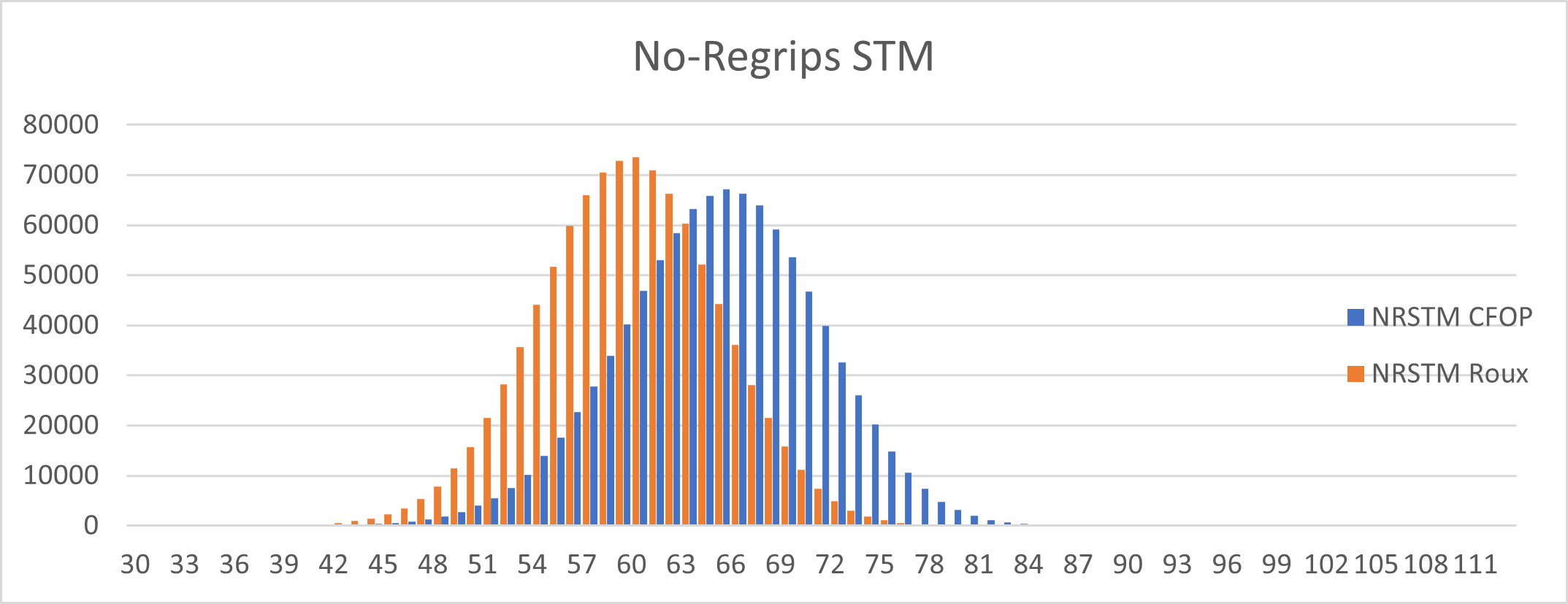
Figure 6. The speeds of CFOP and Roux methods over 1 million solves, measured in slice turn metric, omitting regrips.
As presented above, since CFOP uses less middle slice turns than Roux, under the assumption that the two methods are equal in speed, it is expected that CFOP will generate lower values in all HTMs, and Roux will generate lower values in all STMs.
While the 3 STMs predictably favoured Roux, out of the 3 half turn metrics, only HTM and NRHTM favoured CFOP, while AHTM indicated Roux to be faster. Due to the high number of samples, the p-values evaluated from the two-tailed t-test for all six metrics is effectively 0, and we can visually identify the quicker method from the overlapping distributions.
Table 1. The means and standard deviations in number of moves of CFOP and Roux, measured in the six metrics. T-score is calculated using a paired Student’s T test.
HTM
STM
AHTM
ASTM
NRHTM
NRSTM
CFOP mean
68.905347
67.962297
79.414499
78.471449
66.602106
65.659056
Roux mean
73.609764
64.264263
77.544101
68.198600
68.809291
59.463790
CFOP SD
6.581088
6.904131
6.531167
6.877734
5.661963
5.993907
Roux SD
7.116545
6.163162
7.203812
6.189490
6.428597
5.422036
T-score
485
399
192
1110
257
766
Discussion
The accepted average STM values for CFOP and Roux is 60 and 48 respectively [9] [10], which significantly deviates away from the experimentally obtained values of 68 and 64. This can be explained by the use of adjust U-face techniques [11], which rotate a single face instead of the entire cube to match specific cases; this takes up moves, as opposed to cube rotations, which do not take up moves, but are not widely used in actual speed-cubing, as a single move takes less time than a cube rotation.
The other source of error would be due to the not perfectly optimized intuitive steps. As we have taken an algorithmic approach to simulate these steps, it is likely that it is not the best way to do so. However, since Roux, having two intuitive steps, should be less optimized than that of CFOP, which only has one intuitive step, it is logical to conclude that Roux is quicker than CFOP.
Although the data shown suggests that the Roux method is faster than CFOP, we must keep in mind that different variations can be introduced to both methods, further increasing their efficiency and speed. Realistically, the number of variations we can use is limited by the number of cases and algorithms the cuber can memorize and perform efficiently. At the highest level of speed-cubing, cubers will seldom only use the basic forms of these methods, but rather take the approach of that method, and combine steps from different methods to decrease their solve times.
In addition, there is a historical factor involved. CFOP was first proposed in 1981 [9], but Roux was introduced in 2003 [10]. As a result, CFOP is much more researched, with more variations and algorithms discovered. This leads to a higher popularity among speed-cubers, since a lot more information surrounding CFOP is readily available.
Furthermore, although our data supports the idea that the basic form of Roux is faster than that of CFOP, we cannot recommend CFOP cubers to change over to Roux. This is because at the highest level, variations for both methods will share many algorithms. Therefore, it is unlikely that any one method will have a definite advantage over the other. However, for beginners going into speed-cubing, looking to choose a method, we can suggest Roux as a quicker method than CFOP.
Concluding Remarks
Roux is shown to be quicker than CFOP in 4 metrics out of a total of 6 measured and should be recommended to beginners. However, since speed comes with instinct, not thought, we cannot recommend speed-cubing veterans to change methods after years of practicing and training.
Jargon & Supplemental Information
CFOP (Fridrich’s Method): A speed-solving method whereby the cube is solved in 4 steps. A cross is created on one side, and then an abundance of different algorithms is used to solve the first two layers of the cube simultaneously. The final layer is then solved in two steps, first by correctly orienting those blocks, and then permuting them into the correct position [6].
Roux method: A speed-solving method whereby solvers first focus on solving the corners of the cube through the building of two sets of 1x2x3 blocks, then solve the four remaining corners, and then completing the last six edges [5].
Corner-cutting: The phenomenon in which when a side is not completely aligned, another perpendicular side can still be turned due to the flexible design of cubes. This results in a distinctive “snap” when the unaligned side clicks into place.
Finger-Tricking: An unofficial term employed by competitive cubers whereby cubers solve cubes much more quickly by the ability to turn sides with a single finger movement, rather than the movement of the entire hand [2]. This allows cubers to turn multiple sides simultaneously.
HTM (Half-Turn Metric): A metric for the 3x3x3 Rubik’s Cube where any turn of any face, by any angle, counts as 1 turn [3].
QTM (Quarter-Turn Metric): A metric for the 3x3x3 Rubik’s Cube where any turn of any face by 90 degrees counts as one turn. It differs from the half-turn-metric because half-turns (turning the same face twice) count as two moves instead of one [3].
STM (Slice-Turn-Metric): A metric for the 3x3x3 Rubik’s Cube where any turn of any layer, by any angle, counts as one turn. It differs from the half-turn metric because middle-layer turns count as one move instead of two [3].

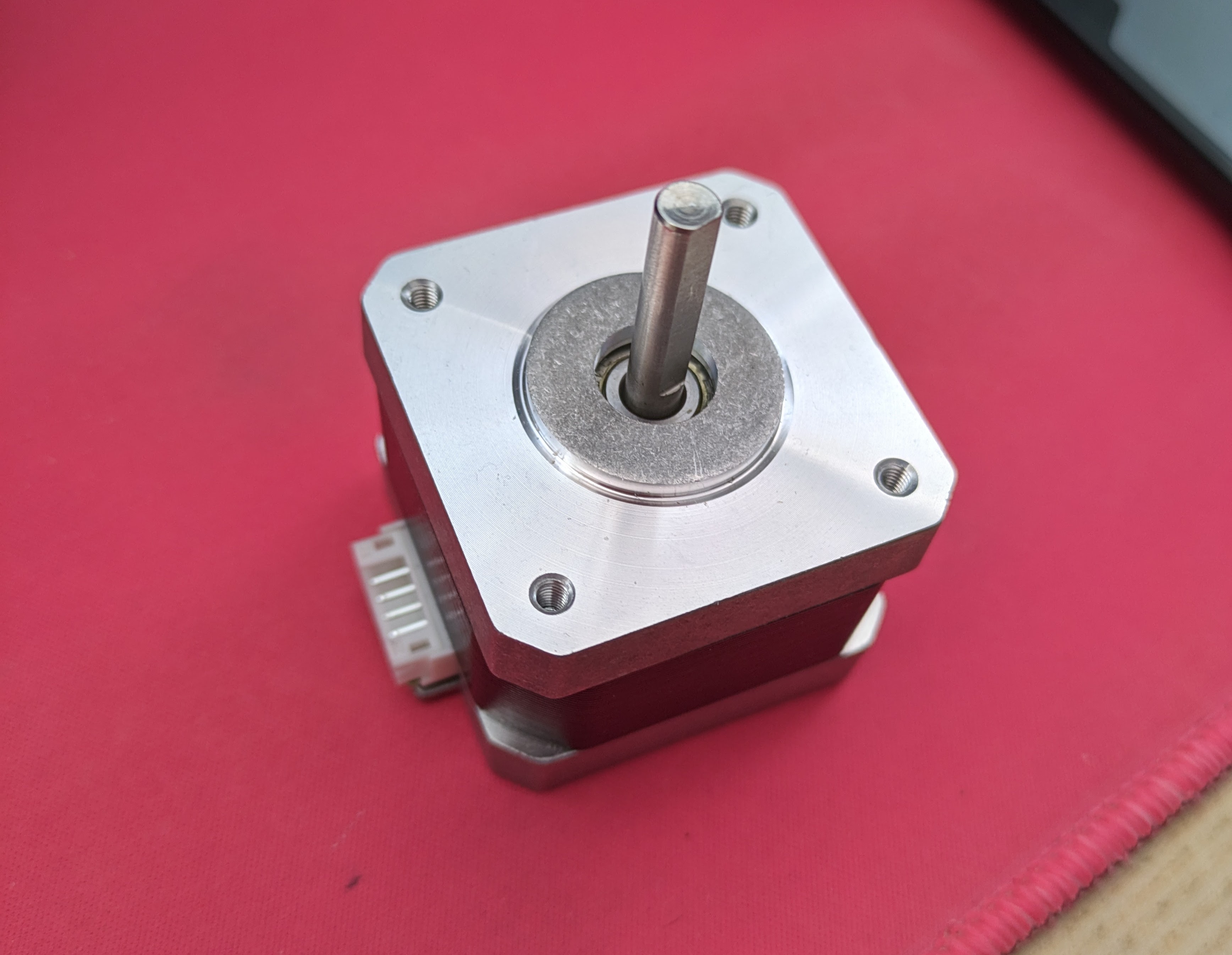
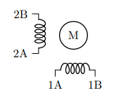
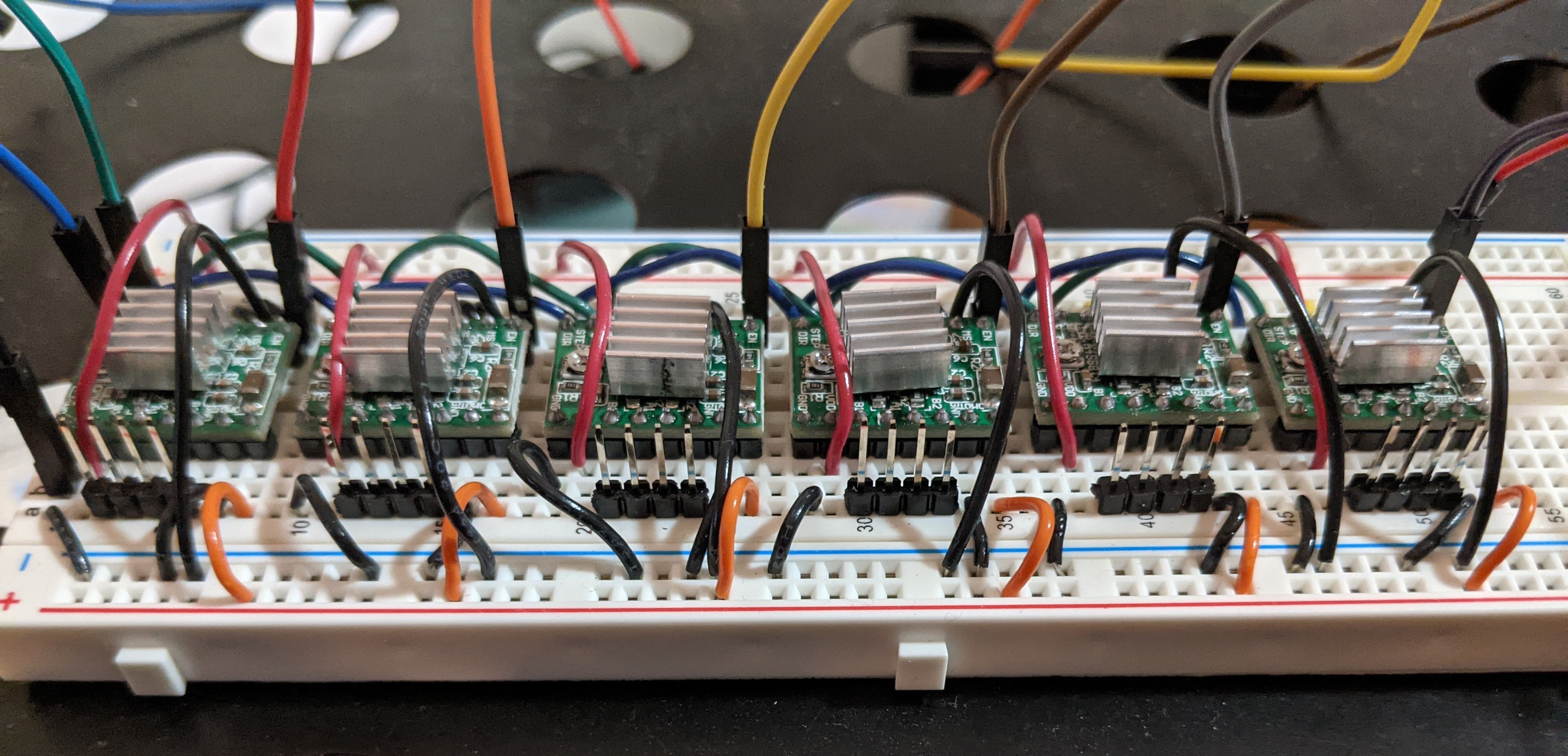
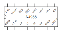
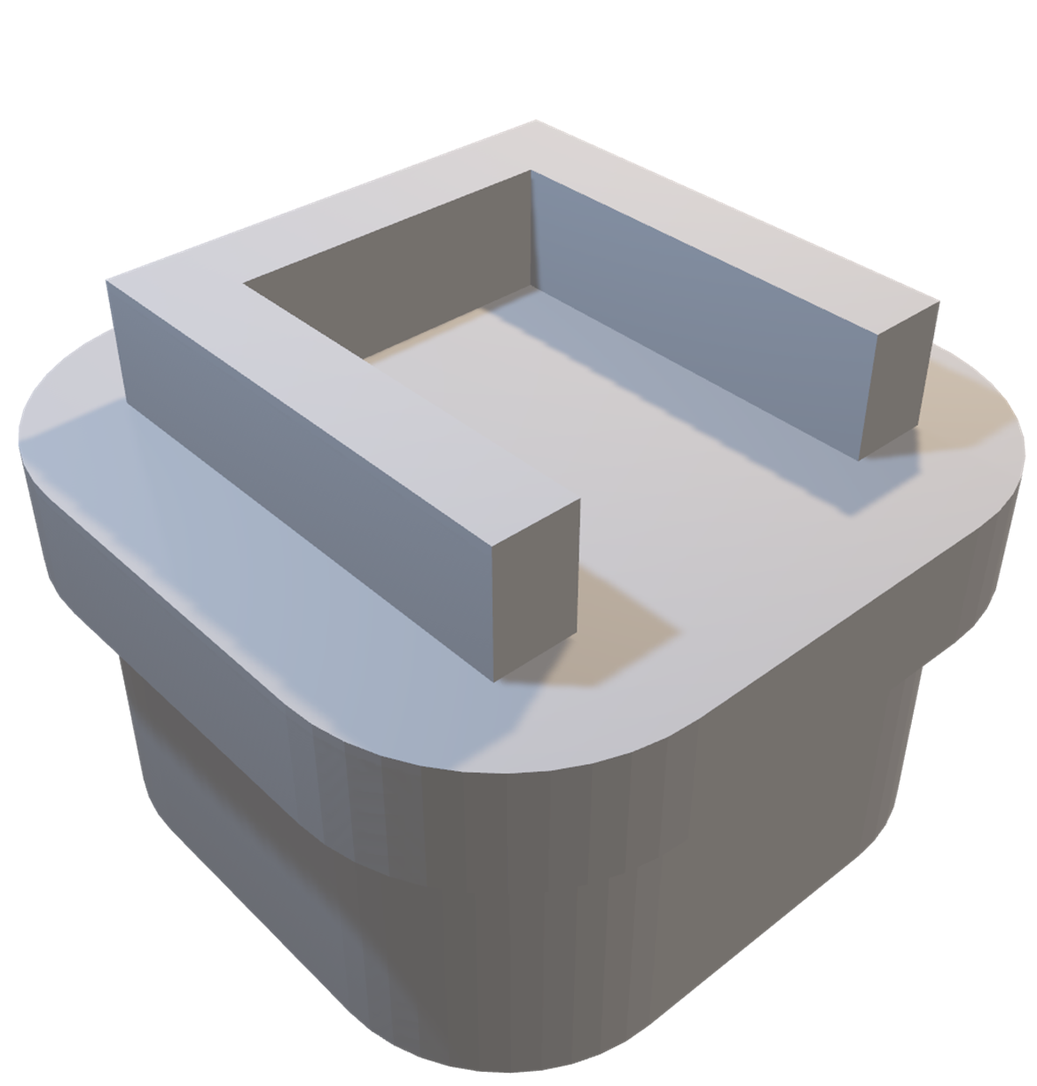

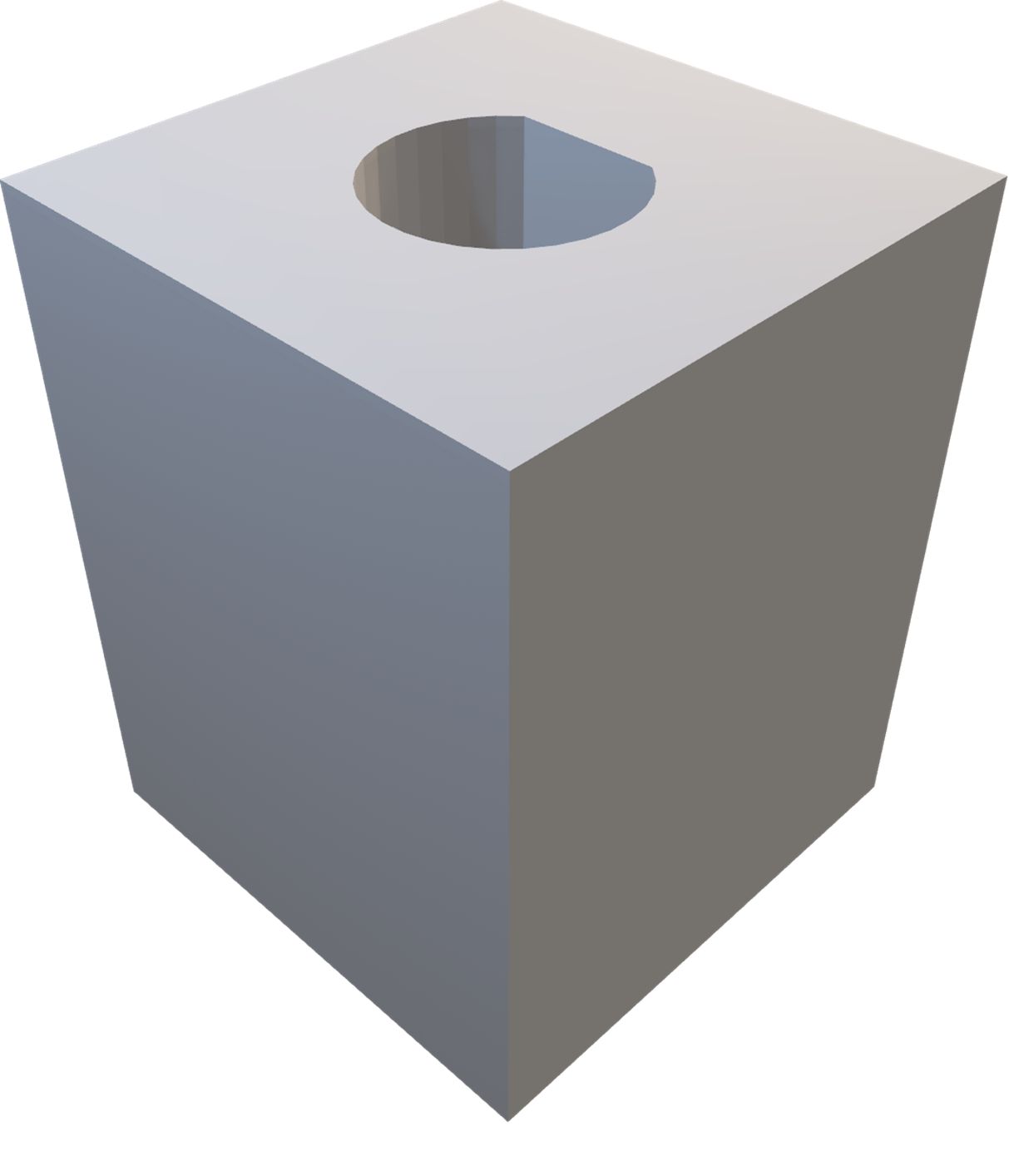
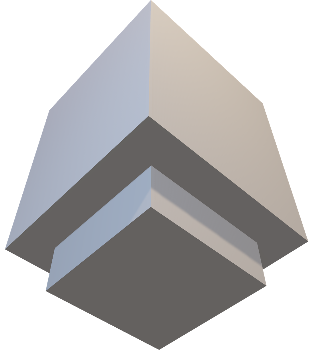
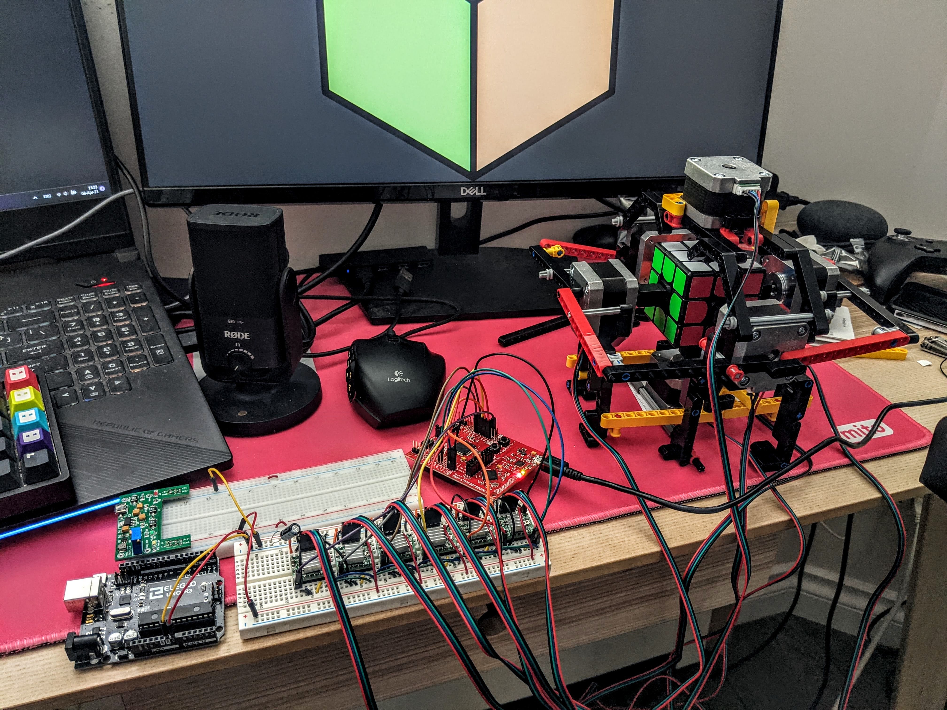
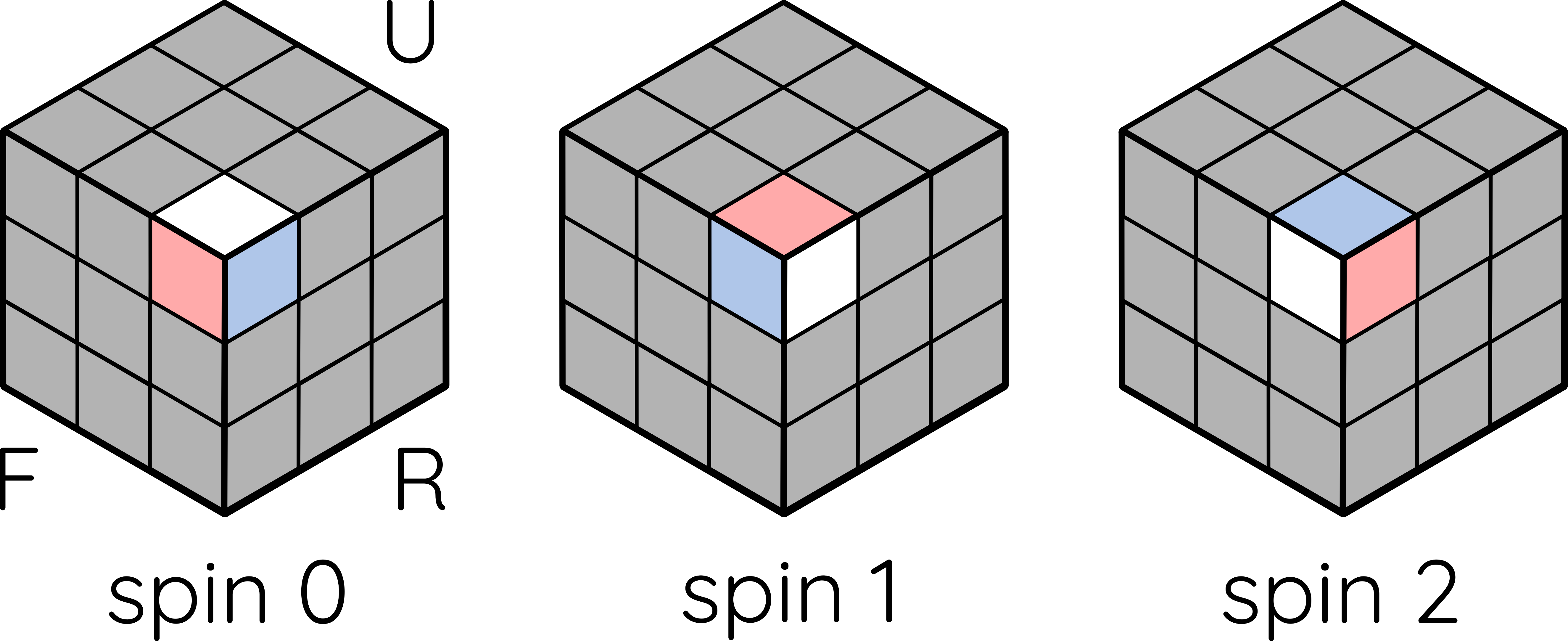
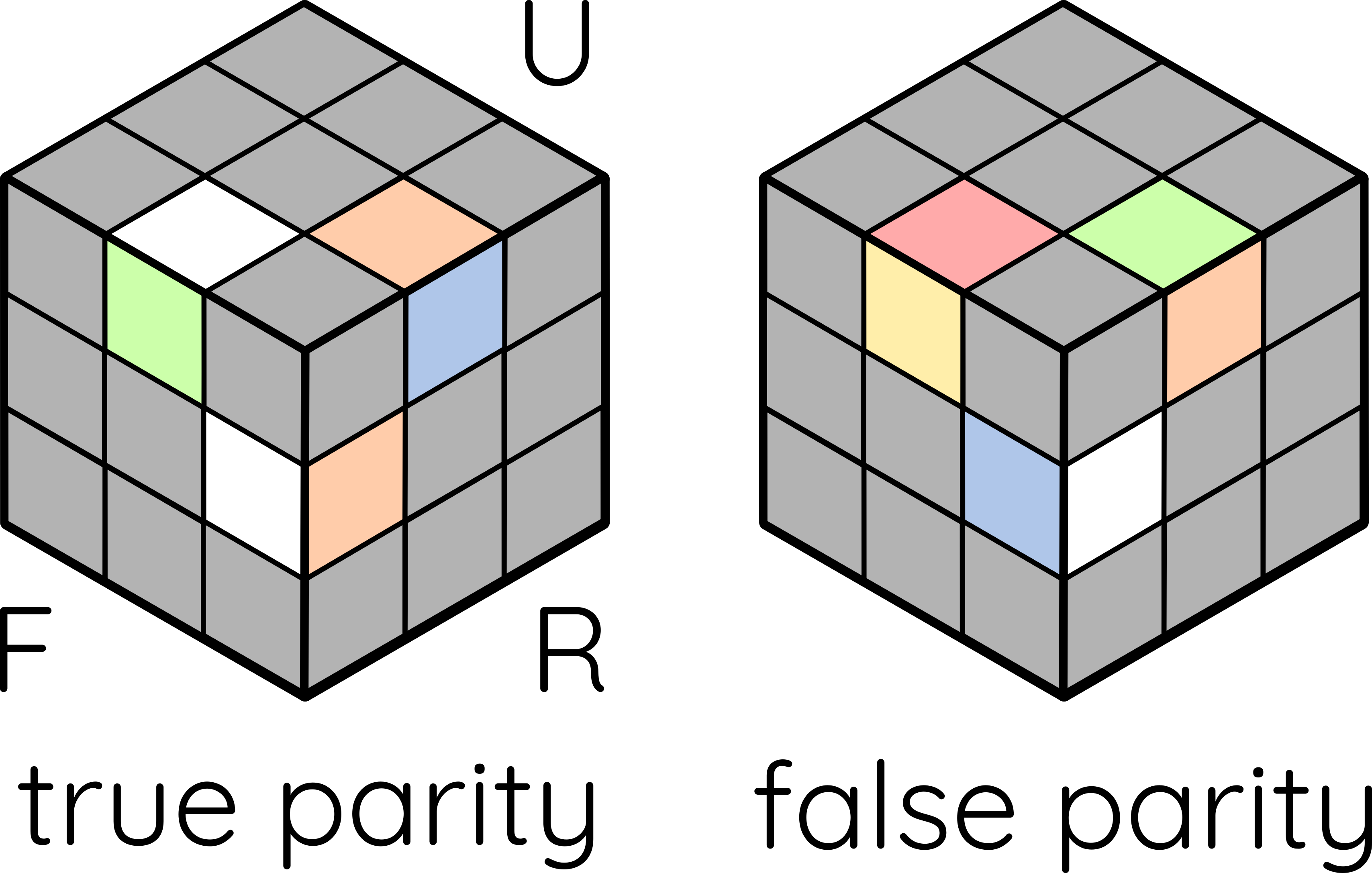
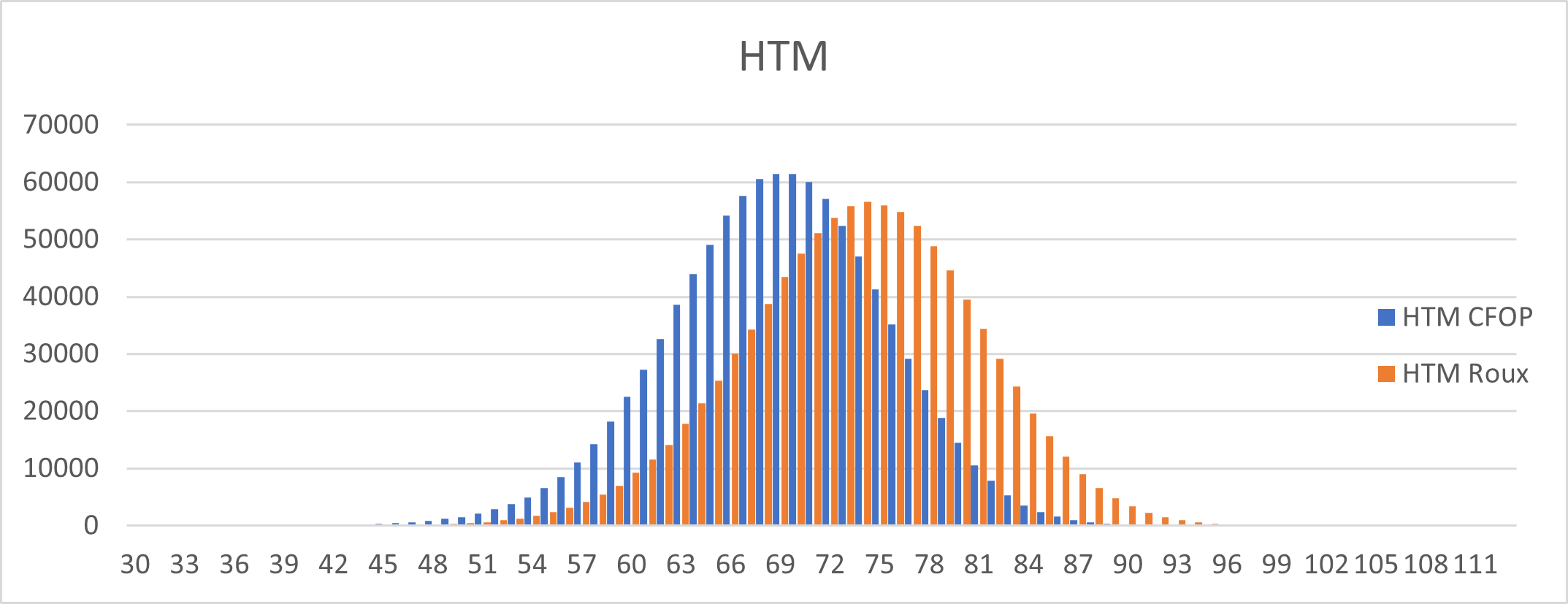 Figure 2. The speeds of CFOP and Roux methods over 1 million solves, measured in slice turn metric.
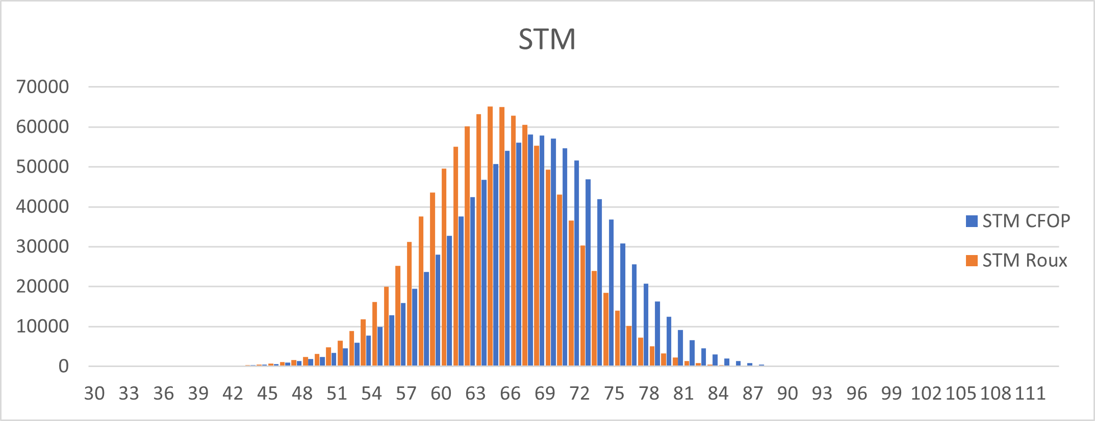 Figure 3. The speeds of CFOP and Roux methods over 1 million solves, measured in half turn metric with adjustment factor.
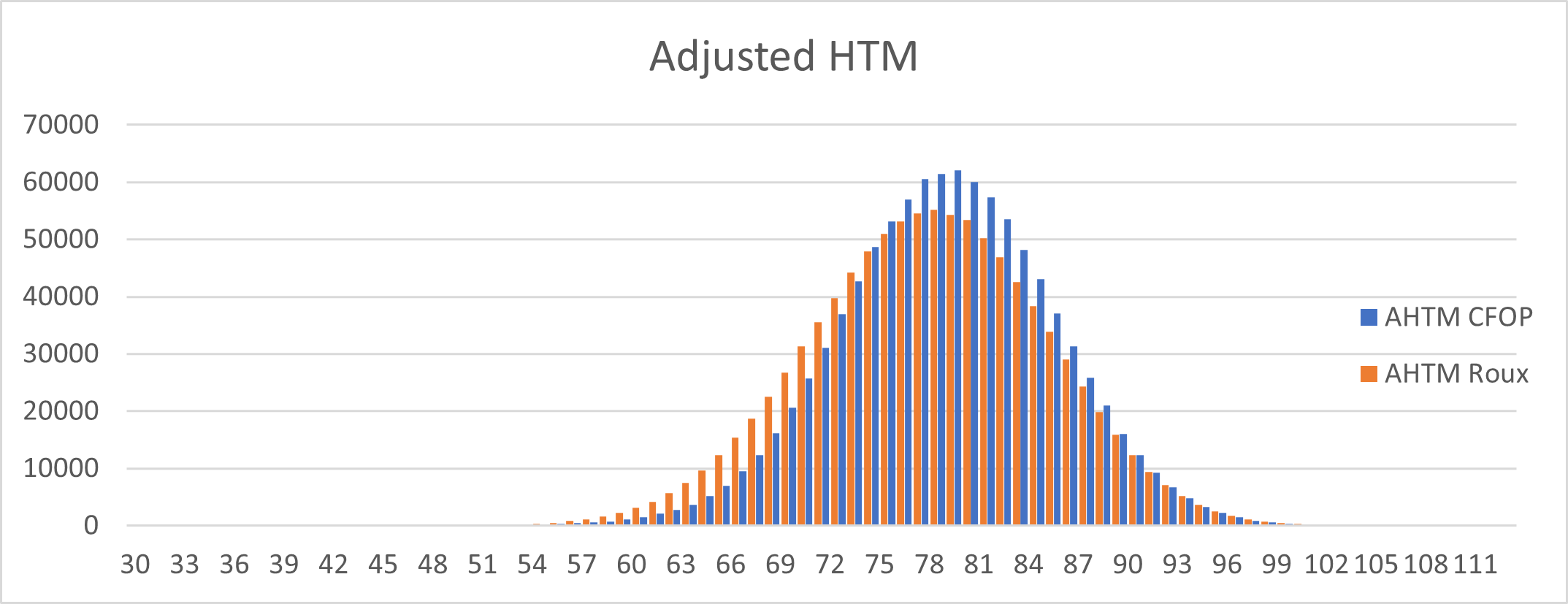 Figure 4. The speeds of CFOP and Roux methods over 1 million solves, measured in slice turn metric with adjustment factor.
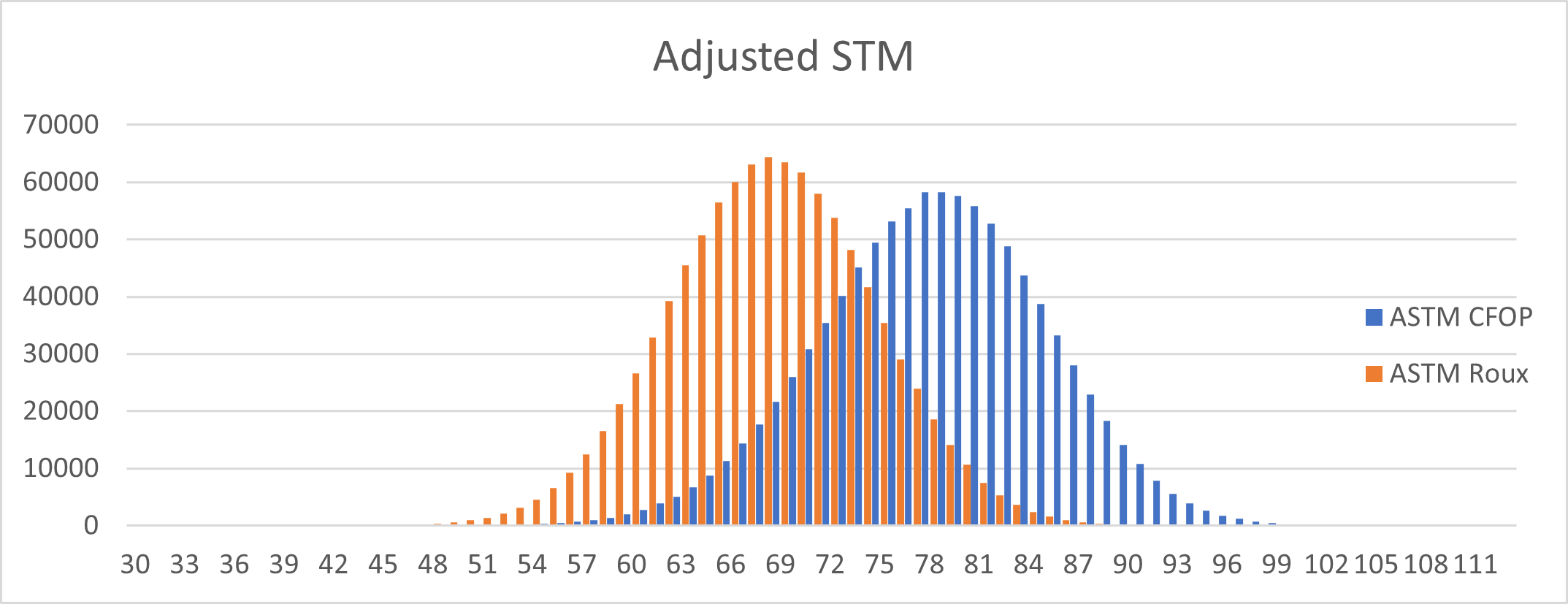 Figure 5. The speeds of CFOP and Roux methods over 1 million solves, measured in half turn metric, omitting regrips.
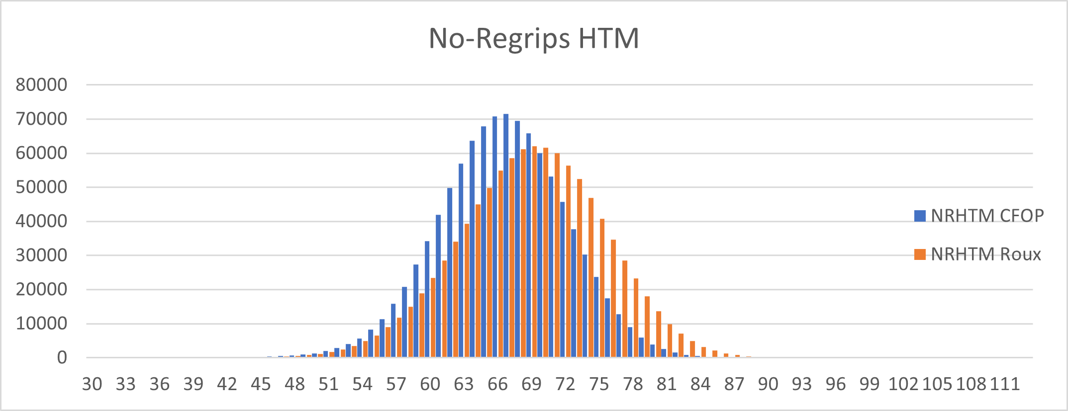 Figure 6. The speeds of CFOP and Roux methods over 1 million solves, measured in slice turn metric, omitting regrips.